Table of Contents

1. Introduction
   • Background / Goal
   • Related Work
2. Approach
   • Dataset
   • Planned Experiments
   • Fixing Imbalances
   • Future Steps
3. Experiments & Results
   • Experiment 1:
   • Experiment 2:
   • Experiment 3:
   • Experiment 4:
   • Experiment 5:
4. Conclusion
   • Recap!
   • Current Limitations
   • Future Work
   • Summary
5. References

Introduction

Surface defect detection is critical in industrial quality control. Manual inspection is slow, inconsistent, and prone to error.

This project uses computer vision to automate detection of metal surface defects. We fine-tune a pretrained ResNet18 model to classify images into 10 defect categories from the GC10-DET dataset.

Goal: given an image of a metal surface, predict the correct defect class accurately and reliably.

Background / Goals

Related Work

Pre-Deep Learning:

Pretty much these are early methods that used handicrafted features (Gabor Filters, LBP) with SVM’s, but mostly struggled to generalize across conditions

ResNet (He et al., 2016):

Introduced a deep residual learning algorithm, which now became the standard backbone for any recent ViT (Vision Transformers) model

Transfer Learning:

This is the practice of using a fine-tuned pretrained CNN model on small industrial datasets

Class Imbalance:

A persistent challenge that rules over GC10-DET (our dataset), that is later addressed via weighted losses and many oversampling strategies

Advanced Detectors:

Recently this comes in the form of: YOLO, R-CNN’s, and ViT for detection tasks

Our Baseline:

If we need a classification with limited data, a fine-tuned ResNet remains a competitive baseline.

Approach

Basically, we took a pretrained ResNet 18 and fine-tuned it for our 10-class problem. Resizing all images to 224x224 and normalize it using ImageNet’s mean and standard deviation; required since it’s what the pretrained weights are expecting.

We then split the data to a 75/15/10 <-> train/val/test split with a fixed random seed for reproducibility. But this brings the issue of handling class imbalances.

We do this by using a WeightedRandomSampler, which oversamples rare classes in each batch. Importantly, we then used an unweighted CrossEntropyLoss since any balances could happen only through the sampler to avoid double-counting.

Therefore, by also training with Adam (an optimizer that adjusts learning rates during training) at a learning rate of 0.001, a batch size of 32, and 25 epochs with the CosineAnnealingLR method to gain metrics such as:

• normalized confusion matrix
• precision/recall/F1
• Cohen’s Kappa

Planned Experiments

To elaborate more, we made three planned experiments at the start of this project!

• Regular Canny Edge Detection - Where we just highlighted surface features (like oil spots, cracks, creases, and other structural anomalies)

• Weld Seam Analysis - Analyzed any weld seams for cracks / incomplete fusions using close-up images. Then applied a Canny Edge Detection model to highlight seam irregularities along those weld lines (to see if it can detect irregularities that might be difficult to spot normally)

• Evaluation Metrics - Maintained a confidence score measuring how close a predicted class is to the TRUE defect type

Really, we intended to use a Canny Edge Detector as a preprocessing step to highlight structural defect features, and then apply it specifically to a weld seam analysis, and track a confidence score as our evaluation metric.

However, as you’ll see later, Experiment 1 directly tests this detection idea (but it didn’t work the way we expected).

Dataset

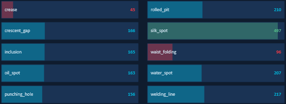
This GC10-DET dataset contains images that are collected in real industrial settings across 10 surface defect classes.

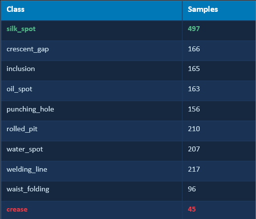
In other words, this dataset contains REAL industrial images across 10 defect classes. As you can see the class imbalance is very severe since “silk_spot” has 497 training images (highlighted in green), while the “crease” class only has 45 training images (highlighted in red). That’s obviously an 11x difference!

Meaning that without any correction, the model would just learn to predict “silk_spot” constantly since that minimizes our loss. Which is WHY the WeightedRandomSampler is super critical!

To see more details -> look in next section!

Splitting the Dataset

Here is the actual code from our program for how we split the data. We first carve out the test set from the full dataset, then split the remaining portion into its train and validation. The fixed generator means anyone running this code will get identical splits.

## USED TO PREVENT OVERFITTING ! ! !
test_ratio = 0.10
val_ratio = 0.15
train_ratio = 1 - test_ratio - val_ratio

generator = torch.Generator()
generator.manual_seed(42)

train_val, test = random_split(
    dataset,
    [train_val_size, test_size],
    generator=generator
)

train, val = random_split(
    train_val,
    [train_size, val_size],
    generator=generator
)

Fixing The Imbalances

THE PROBLEM: Our initial model attempts had very poor per-class accuracy because the silk_spot class (497 images) had vastly outnumbered the crease class (45 images). The model defaulted to predicting majority classes.

The Fix: Get a WeightedRandomSampler! This is because it assigns each training sample a weight that is inversely proportional to its class size. Therefore, rarer classes are oversampled and common classes are undersampled. Which is then balanced through the sampler, not also through the loss function, to avoid double-counting.

Future Steps

Giving way to our roadmap:

• Training & Monitoring - Where we train across multiple epochs, track loss curves, and save its best performance as a checkpoint.

• Confusion Matrix Eval - Evaluate performance using a normalized confusion matrix on the held-out test set.

• Hyperparameter Tuning - Tune learning rate, batch size, and optimizer settings to improve accuracy.

• Data Augmentation - Improve generalization across oil spots, cracks, creases, and other defect types.

• Stronger Backbone - Experiment with ResNet50 or EfficientNet for enhanced feature extraction.

• Weld Seam Analysis - Apply Canny edge detection to close-up weld images to detect anomalies along seam lines.

• Real-World Deployment - Validate accuracy against live defect samples in a factory environment.

Leading to most of these becoming part of our experiments

Experiments & Results

Experiment 1: Canny Preprocessing Ablation

What we did: Applied Canny edge detection (thresholds 100/200) as preprocessing. Replaced original RGB images with binary edge maps before feeding into ResNet18.

Purpose: Test if explicit edge features improve defect classification.

Result: 41% test accuracy.

Insight: Edge maps removed texture and color information. This broke compatibility with ImageNet pretrained weights.

Decision: Removed Canny from training. Used only for visualization.

Experiment 2: Class Balancing Strategy

Whlie our initial implementation applied both WeightedRandomSampler and a weighted CrossEntropyLoss simultaneously. Both mechanisms are trying to solve the same problem — make the model treat rare classes fairly. Using both at once means the correction is applied twice, causing the model to over-correct and treat rare classes as far more important than they actually are.

Initial (Wrong): Applied both WeightedRandomSampler AND weighted CrossEntropyLoss simultaneously.

Fixed Approach: WeightedRandomSampler that only resamples batches without modifying the loss — no double-counting.

Experiment 3: Training Duration and Learning Rate Schedule

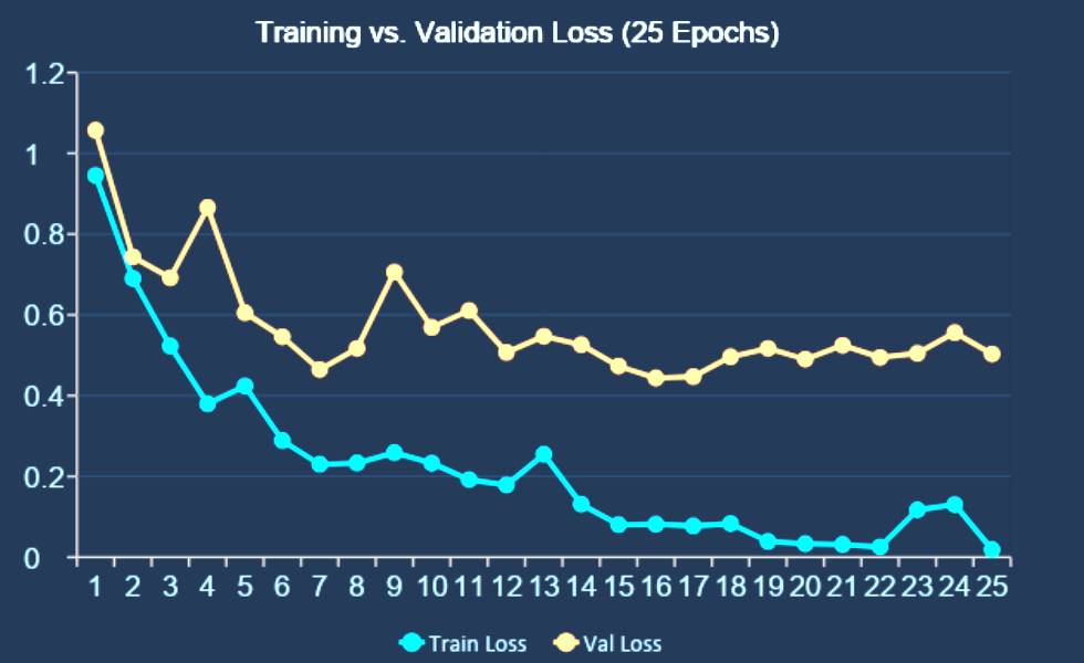
Setup: Adam optimizer (lr = 0.001) with CosineAnnealingLR over 25 epochs.

Key observations:

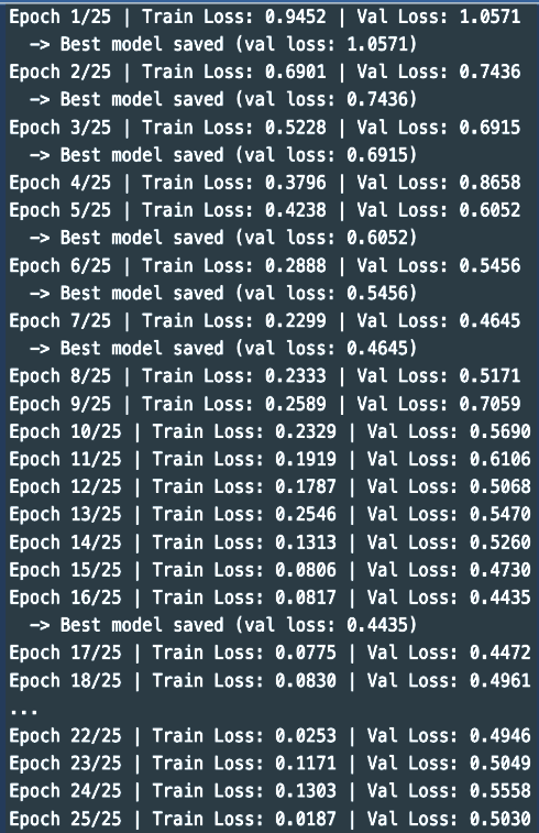
• Epoch 1: Train loss 0.945, Val loss 1.057
• Epoch 7: Early best (Val 0.465)
• Epoch 16: Best checkpoint (Val 0.444)
• Epoch 25: Train loss 0.019, convergence reached

Insight: Longer training with learning rate decay improved convergence and final performance.

Experiment 4: Final Test Set Evaluation (n = 256)

On 256 test images, we hit 88% accuracy, a Cohen’s Kappa of 0.859, and a Macro F1 of 0.85.

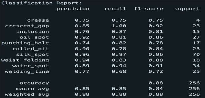
Insight: silk_spot is the strongest class at F1 = 0.96. welding_line is the weakest at F1 = 0.72, likely due to visual overlap with other surface irregularities.

Experiment 5: GradCAM Spatial Localization

GradCAM gives us a way to see where the model is looking. We hook into layer4[1].conv2, the last convolutional layer of ResNet18, register forward and backward hooks, backpropagate the predicted class score to get gradient tensors, global-average-pool those gradients to get per-channel importance weights, then take a weighted sum of the activation maps, apply ReLU, normalize to [0,1], and __overlay the heatmap on the original image.

How It Works:

• Hook - Registers forward + backward hooks on layer4[1].conv2
• Gradient - Backpropagates predicted class score to get gradient tensors
• Weight - Global average pools gradients over spatial dims -> per-channel importance weights
• Map - Weighted sum of activation maps -> ReLU -> normalize to [0, 1]
• Overlay - Heatmap upsampled and blended onto the original RGB image for visualization

Demo Results:

• Class: water_spot | Confidence: 100.0% -> Heatmap correctly highlighted defect region. High confidence, correct localization.
• Class: welding_line | Confidence: 40.9% -> Correct prediction but has low confidence; causing it to be the weakest class in the dataset.

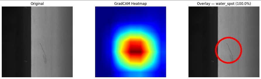
^shown is an example of water_spot in GradCAM^

Basically, this is a the GradCAM heatmap where it just shows the model’s attention! Mostly concentrating on the center-right where the defect is, overlaying it with a red circle that marks the localized region.

Conclusion

We identified three main issues that limited performance:

• Canny preprocessing removed important image information
• Double class balancing caused unstable training
• Too few epochs prevented convergence

After fixing these:

• 88% test accuracy
• 0.859 Cohen’s Kappa

The final ResNet18 model performs well across all 10 defect classes.

Recap!

We started with a baseline using ResNet18 that achieved only 41% accuracy due to three compounding issues: Canny preprocessing corrupted pretrained features, a double class that balanced over-corrected imbalances, and too few epochs that prevented convergence.

However, after diagnosing and fixing each issue, the final model achieved an 88% accuracy with a Cohen’s Kappa of 0.859 across ALL 10 defect classes.

Limitations

• welding_line weakness - F1 = 0.72, the lowest class, which is likely due to visual overlap with other surface irregularities.

• crease fragility - Only 4 test samples -> a single prediction flip that changed F1 significantly.

• Benchmark-only evaluation - The GC10-DET dataset is clean since real factory conditions add variation in lighting, noise, and co-occurring defects.

Future Work

• welding_line sub-classifier - Dedicated binary classifier or targeted augmentation for the weakest class.

• Deeper backbone - ResNet50 or EfficientNet for finer texture discrimination.

• Out-of-distribution testing - Evaluate on real manufacturing data to measure generalizability.

• Edge deployment - Quantize / prune model for inference on factory hardware.

Summary

In actuality, ResNet18 was fine-tuned on a GC10-DET dataset that achieved an 88% accuracy and Kappa 0.859 across 10 steel surface defect classes.

After resolving Canny preprocessing corruption, double class-balancing, and insufficient training depth. The model correctly localizes defect regions via GradCAM. The main contribution is identifying and resolving three specific failure modes that together accounted for a 47-point accuracy gap.

References

• Lv et al. (2020). Deep Metallic Surface Defect Detection: The New Benchmark and Detection Network. IEEE Access.
• He et al. (2016). Deep Residual Learning for Image Recognition. CVPR.
• Deng et al. (2009). ImageNet: A Large-Scale Hierarchical Image Database. CVPR.
• Buda et al. (2018). A Systematic Study of the Class Imbalance Problem in CNNs. Neural Networks.